Detection of DNA Looping Interactions
Introduction
CHiCAGO (Capture Hi-C Analysis of Genomic Organisation) is the most common tool for the detection of DNA looping interactions in capture Hi-C data. The underlying assumption of the approach is that background signal is the result of Brownian noise (distance dependent with a negative binomial distribution) and Poisson distributed technical noise. Signal that is higher than the background is considered a result of significant interactions, such as in the case of P-E interactions.
Please note that the entire analysis approach that we describe here is bait based and not probe based, meaning all probes of the same promoter are pooled together and interactions called at the bait level (see the main page to refresh your memory on the difference between probes and baits). If you are interested in analyzing the data in a probe-centric approach you will need to adjust the steps below. This will also require much higher sequencing coverage as CHiCAGO requires, by default, a minimum of 250 reads per captured fragment.
Installing CHiCAGO package and CHiCAGO tools
Please install CHiCAGO from this forked repository (includes minor bug fixes) as follows:
git clone https://github.com/dovetail-genomics/chicago.git
And install the R package (and its dependencies, if not already installed; requires R version >= 3.1.2.).
In your R console:
install.packages("argparser")
install.packages("devtools")
library(devtools)
install_bitbucket("chicagoTeam/Chicago", subdir="Chicago")
Input files
Genomic fragments and design directory
CHiCAGO requires as an input two sets of genomic intervals:
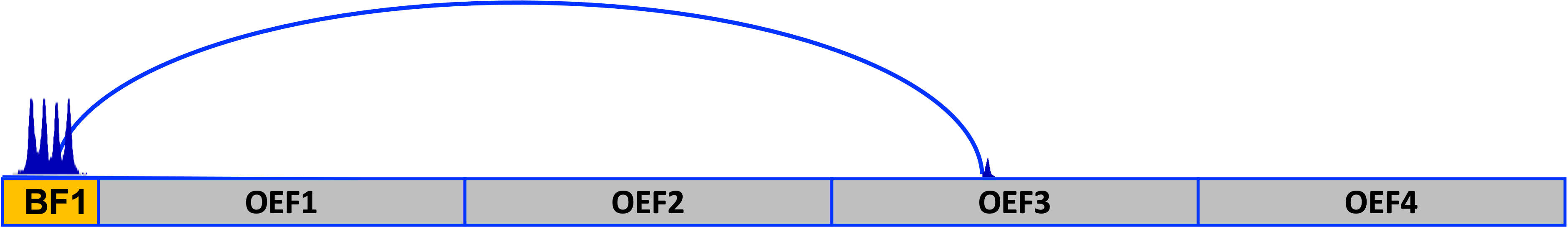
Bait Fragments (BF) - fragments overlapping baits
Other End Fragments (OEF) - all other genomic fragments to be included in the analysis
In the example below, you can see the two types of fragments, BF (in orange) and OEF (in gray). The locations of the BF and OEF are required as an input (more details below). In this example, an interaction detected by CHiCAGO between BF no.1 and OEF no.3 is depicted.
Here, since RE-free methods are used (Omni-C® or Micro-C® assays), DNA can be fragmented at almost any position. To generate the OEF we simply bin the genome at the desired window size (e.g. 10 kb). The final OEF set is composed of all the binned intervals that do not intersect with the BF set. To generate BF intervals, probes of the same gene are pooled together (usually covering about 2 kb) into one fragment (and in some cases, if overlap occurs, probes of two genes may be pooled into a single fragment).
The OEF and BF are captured in .rmap and .baitmap files, and are used to generate additional design files that are required for CHiCAGO. For your convenience we have generated all design files needed to be used with CHiCAGO. These can be found in the data-sets section. If you are interested in generating the files on your own, please review the For advanced users section at the bottom of this document.
We recommend starting with 10 kb (size of OEF fragment size, labeled h_10kDesignFiles for human or m_10kDesignFiles for mouse). Design files with 5 kb, 10 kb and 20 kb are provided (data-sets section).
Download the desired CHiCAGO design directory and uncompress it:
wget https://s3.amazonaws.com/dovetail.pub/capture/human/CHiCAGO_files/h_10kDesignFiles.tar.gz
tar xzvf h_10kDesignFiles.tar.gz
10 kb typically works well with libraries of 150 M read-pairs or more. However, if the number of reads fall below that value (or if the library is of lower quality, e.g. due to high dup rate) 20 kb may be a better choice. For better resolutions (5 kb and even 2 kb), higher sequence coverage is required (thids can be achieved by sequencing more or by pooling together multiple replicas as will be discussed below). A good practice would be to start with 10 kb, and, after reviewing the CHiCAGO results, consider whether to rerun with alternative fragment size.
chinputs
The mapping information to be used as input for identifying significant interactions needs to be adjusted to the CHiCAGO format, named chinput. To generate chinput files you will need the .rmap and .baitmap from your chosen design files directory and the CHiCAGO compatible bam file. The bam2chicago.sh script is used to generate input files (chinput) using your choice of design files.
Create chinput files:
Important!
Make sure to use the CHiCAGO compatible bam file such as chicago.bam from the From fastq to bam files section
Command:
./chicago/chicagoTools/bam2chicago.sh <capture.bam> <baitmap> <rmap> <output_prefix>
Example:
./chicago//chicagoTools/bam2chicago.sh chicago_capture_NSC_rep1.bam \
./h_10kDesignFiles/pooled_10kb_120bp.baitmap \
./h_10kDesignFiles/digest10kb_pooled120bp.rmap \
10kb_chinput_NSC_rep1
The output following the above example is a new directory, 10kb_chinput_NSC_rep1, with the desired chinput, file 10kb_chinput_NSC_rep2.chinput, that will be used in the next steps for running CHiCAGO. The output directory also includes a bait2bait*bedpe* file with pairs overlapping baits at both ends of the pair. We will not use this file in our analysis.
 Generating chinput files is the most time-consuming step in the CHiCAGO pipeline, taking about 1.5 hours for a dataset with 250 M read-pairs on an Ubuntu 18.04 machine with 16 CPUs, 1TB storage and 64GB memory.
Interaction calling
Now that you have all the needed input files, you can run CHiCAGO to obtain a list of significant interactions. Chinputs from one replica or more can be used. As mentioned above, we recommend using the 10 kb design files for initial interaction calling. Depending on your goals and the quality and depth of your data, you may choose to experiment with other fragment sizes.
Parameter |
Value |
Details |
|---|---|---|
--design-dir |
Path to the design directory |
|
--cutoff |
5 |
Score threshold for calling significant interactions (typically set to 5). Scores are calculated as -log weighted p-values based on the expected true positive rates at different distance ranges (estimated from data). Increasing the cutoff will increase the stringency and less interactions will be called. |
--export-format |
Multiple formats are available for exporting the interactions. You can specify multiple formats to be used. We recommend the following: |
|
interBed |
Each interaction detailed as one row with the following fields: bait_chr, bait_start, bait_end, bait_name, otherEnd_chr, otherEnd_start, otherEnd_end, otherEnd_name, N_reads, and score |
|
washU_text |
Can be read by the WashU browser. Upload to the browser using: Tracks → Local Text Tracks → long-range text |
|
washU_track |
Can be read by the WashU browser. Upload to the browser using” Tracks → Local Tracks → longrange (both track file and index file should be uploaded) |
|
seqMonk |
Each interaction is represented by two rows: bait row followed by other-end row. Includes the following fields: chromosome, start, end, name, number of reads and interaction score |
|
<path_to_chinput> |
Path to chinput file(s). If you wish to run CHiCAGO on multiple replicas together, you can specify multiple chinput files ( in a comma separated format). All the chinput files should be made using the same settings and with thesame rmap and baitmap files located in the specified design directory |
|
<output_prefix> |
Command:
Rscript ./chicago/chicagoTools/runChicago.R --design-dir <path_to_design_dir> \
--cutoff 5 \
--export-format interBed,washU_text,seqMonk,washU_track \
<path_to_chinput> \
<output_prefix>
Example, one chinput file:
Rscript ./chicago/chicagoTools/runChicago.R --design-dir ./h_10kDesingFiles \
--cutoff 5 \
--export-format interBed,washU_text,seqMonk,washU_track \
.10kb_chinput_NSC_rep1/10kb_chinput_NSC_rep1.chinput \
NSC_rep1_chicago_calls
Example, chinput files from two replicas:
Rscript ./chicago/chicagoTools/runChicago.R --design-dir ./h_10kDesingFiles \
--cutoff 5 \
--export-format interBed,washU_text,seqMonk,washU_track \
.10kb_chinput_NSC_rep1/10kb_chinput_NSC_rep1.chinput, .10kb_chinput_NSC_rep2/10kb_chinput_NSC_rep2.chinput \
NSC_chicago_calls
Output files
CHiCAGO outputs will be saved to 4 different directories:
Diagnostic plots directory (diag_plots)
This will include 3 diagnostic plots:
The distance plot
Brownian factors
Technical noise estimates
The CHiCAGO Vignette reviews these plots and offers guidance on how to interprete them. If reviewing the diagnostic plots brings you to the conclusion that the results are not ideal (e.g. the curve of the distance plot poorly matches the data points), consider generating new chinputs with 20 kb OEF (instead of the recommended 10 kb) and rerun CHiCAGO. There are also more advanced options for fine tuning CHiCAGO runs that are out of the scope of this documentation (such as re-estimating the P-value weights using the fitDistCurve.R script of chicagoTools). Please refer to the CHiCAGO publication, its bitbucket repository and the CHICAGO vignette for more details and ideas.
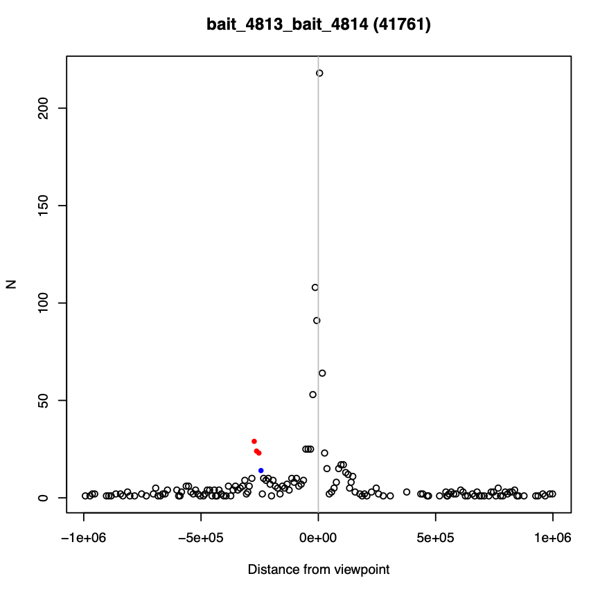
Examples directory (examples)
In this directory, 16 random baits are shown with their associated raw reads (up to 1 Mb from the bait). Interactions above the threshold (default 5) are shown in red, interactions with score 3-5 are shown in blue, and interactions with a score below 3 are in black (see example below). You can also choose to plot specific baits of interest (more on that in the interactions analysis section).
Data directory (data)
This is the main directory you will use for further data analysis.
The output will include all the specified export formats (--export-format, see table above and the CHiCAGO Vignette) as well as R database file (with an extension .Rds) and an interBed file (.ibed extension).
The ibed file is the main file that you will use to analyzeing the detected interactions. The ibed file contains 10 columns:
Columns 1-4 (chr, start, end, bait name) define the bait side of the interaction.
Columns 5-8 (chr, start, end, OE name) define the other end (OE) of the interaction. In some cases, interactions between two bait regions are called, in which case the name of the second bait will be recorded on column 8 (otherwise there is no OE name and it will be marked with
.).Column 9-10 (no. of pairs, score) define the number of pairs that support the interaction call and the associated score. Only interactions above the cutoff are recorded in the .ibed file, but the full data, including interactions with lower scores, are saved in the .Rds database.
Tip
Filter out trans interactions, too short interactions (e.g. < 10 kb) and too long interactions (e.g. > 2 Mb). Here is a simple awk command for filtering the .ibed file:
awk  'NR>1 {if (($1 == $5) && \
(($6 > $3 && ($6 -$3) < 2000000) || ($6 < $3 && ($2 -$7) < 2000000)) && \
(($6 > $3 && ($6 -$3) > 10000) || ($6 < $3 && ($2 -$7) > 10000))) \
print}' <interactions.ibed> >filtered_interactions.ibed
In the NSC rep1 example, 57,194 interactions were called with 52,411 of them passing the above filtering criteria.
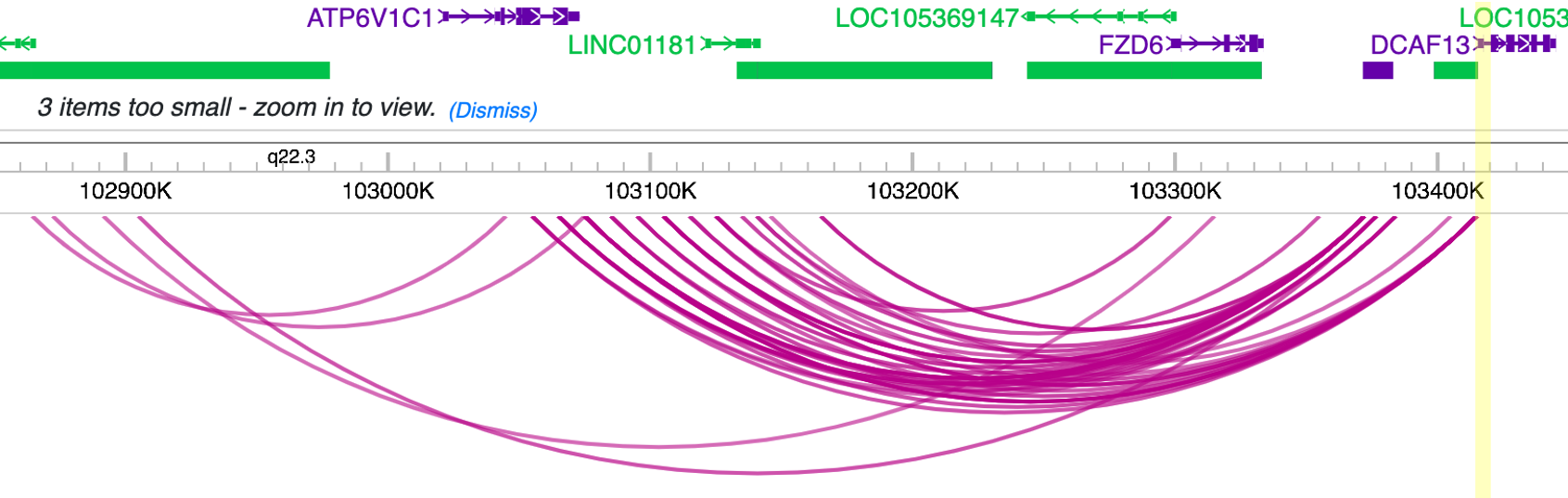
As an example, let’s inspect interactions that involve the DCAF13 promoter as detailed (header line was added for convenience):
bait_chr bait_start  bait_end    bait_name               otherEnd_chr   otherEnd_start otherEnd_end   otherEnd_name  N_reads  score
chr8     103413593   103416224   bait_39283_bait_39284   chr8           103050000      103060000      .              23       6.41
chr8     103413593   103416224   bait_39283_bait_39284   chr8           103060000      103070000      .              24       6.62
chr8     103413593   103416224   bait_39283_bait_39284   chr8           103070000      103080000      .              44       13.75
chr8     103413593   103416224   bait_39283_bait_39284   chr8           103080000      103090000      .              27       7.34
chr8     103413593   103416224   bait_39283_bait_39284   chr8           103090000      103100000      .              24       6.15
chr8     103413593   103416224   bait_39283_bait_39284   chr8           103100000      103110000      .              39       10.99
chr8     103413593   103416224   bait_39283_bait_39284   chr8           103110000      103120000      .              27       6.78
chr8     103413593   103416224   bait_39283_bait_39284   chr8           103120000      103130000      .              23       5.32
chr8     103413593   103416224   bait_39283_bait_39284   chr8           103141449      103150000      .              24       5.3
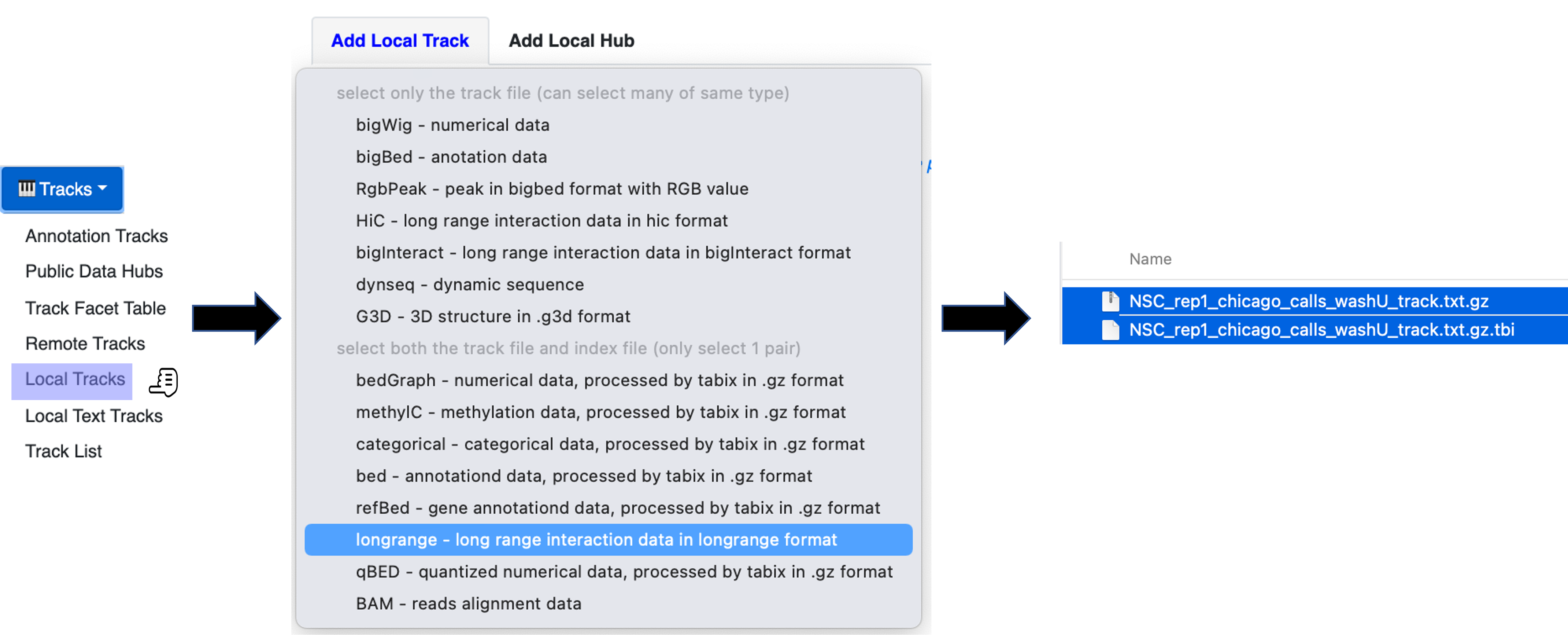
We can also visualize these interactions by uploading the track file to Wash-U browser:
Tip
To visualize interactions on the Wash-U
Under the Tracks menue, choose the option Local Tracks
From the list of track types, choose longrange
3. Choose from the data directory two files together: the file labeled as *washU_track.txt.gz and its associated file *washU_track.txt.gz.tbi (e.g. NSC_rep1_chicago_calls_washU_track.txt.gz and NSC_rep1_chicago_calls_washU_track.txt.gz.tbi)
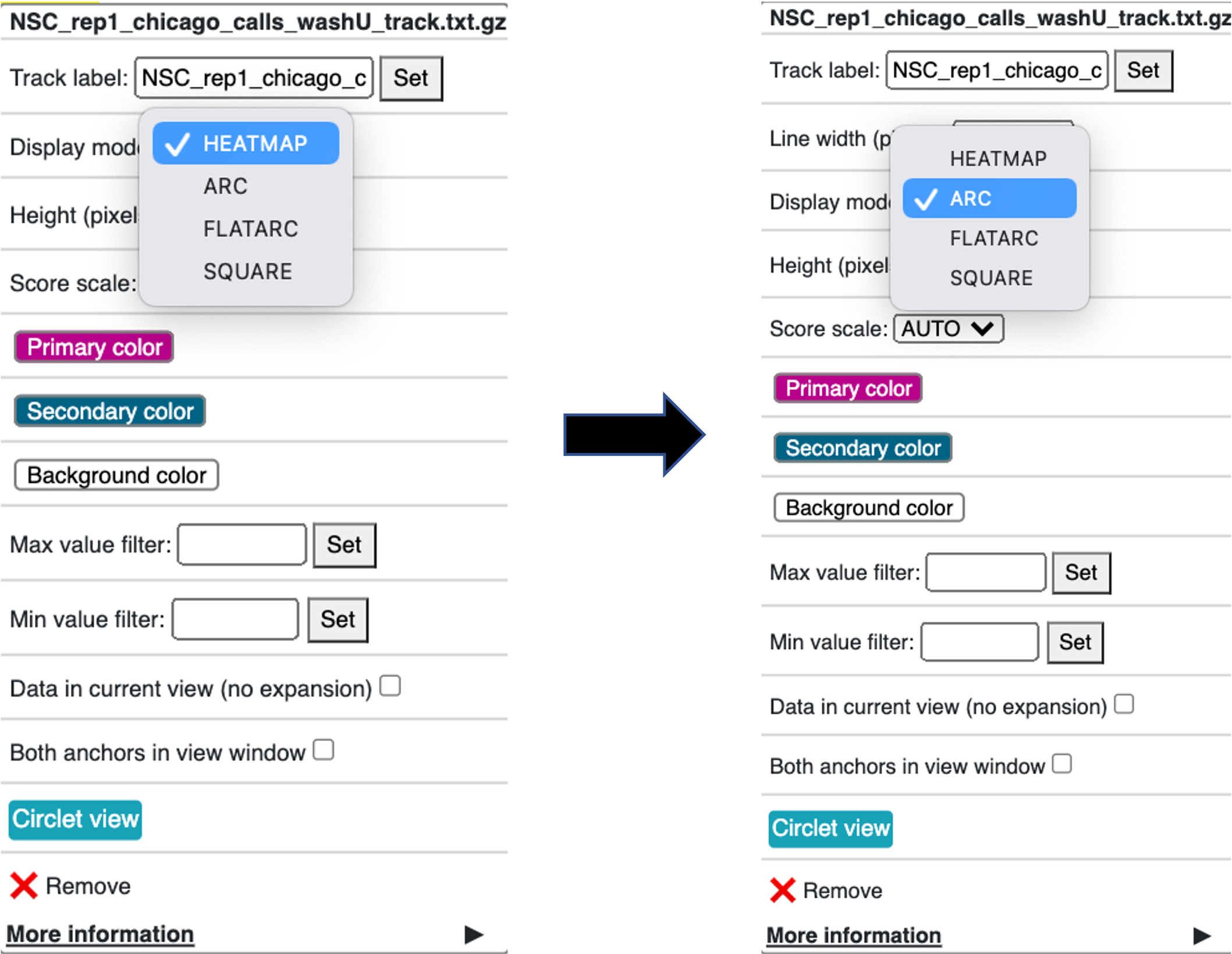
Right click on the new track that was added to the genome browser
Change the Display mode from HEATMAP (default) to ARC
Choose your region of interest to inspect the interactions
Optional - Enrichment plots directory (enrichment_plots)
By default, this directory is empty. However, if you already have position information of different genomic features of interest, CHiCAGO has a built-in feature to estimate if these regions are enriched in the OE side of the detected interactions. Click here for more details.
Typically, we expect the promoter interactions to be enriched for specific genomic features, like CTCF biding sites, specific histone marks, etc. If you want to use CHiCAGO to calculate fold enrichment for genomic regions, gather the bed files (e.g. chip-seq narrow-peak files) and list the feature names and file locations in a tab delimited text file as in the example below. For demonstration, we will name this file genomic_features.txt.
genomic_features.txt:
CTCF  /home/user/data/CTCF.bed
H3K4me1  /home/user/data/H3K4me1.bed
H3k27ac  /home/user/data/H3k27ac.bed
You will also need to specify the option --en-feat-list followed by a direct path to the genomic feature file location (e.g. ./genomic_features.txt) when running CHiCAGO, as in this example:
Rscript chicago/chicagoTools/runChicago.R --design-dir ./h_10kDesingFiles \
--cutoff 5 \
--export-format interBed,washU_text,seqMonk,washU_track \
--en-feat-list ./genomic_features.txt \
.10kb_chinput_NSC_rep1/10kb_chinput_NSC_rep1.chinput \
NSC_rep1_chicago_calls
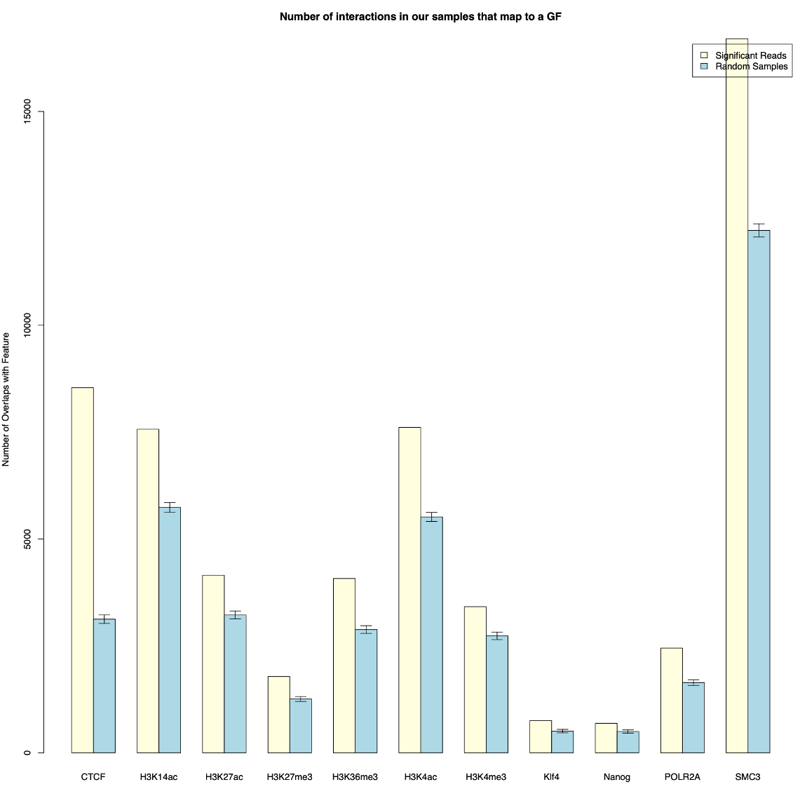
Under the enrichment_plots directory, you will find an enrichment plot, as in the example below, showing how many OE fragments overlap with each genomic feature, and how many would have overlapped as a result of random shuffling of the genomic feature across the genome. The data that was used to generate the plot is also found in the enrichment_plots directory (as a .txt file).
Additional suggestions for interactions data analysis:
TADs - Calculate how many of the interactions are within TADs vs across TADs. We anticipate that a significant majority of the interactions will be within TADs.
A/B compartments - How do the interactions segregate between A/B compartments? Typically, more interactions will be observed in active regions, enriched with open chromatin. These open regions can be detected using ATAC-seq or or inferred through RNA-seq experiments.
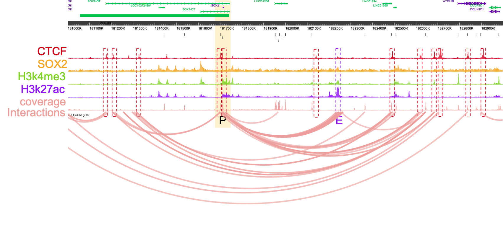
Overlay the information from your experiment with additional data types such as RNA-seq, Chip-seq or existing databases of regulatory elements, either for enrichment studies or for exploring specific promoter regions. In the example below you can see how the majority of the interactions associated with the SOX2 promoter co-occur with CTCF Chip-seq peaks:
GO analysis and motif enrichment studies are also potential exploration paths.
In most cases, users will have datasets from multiple sample types (e.g. different cell lines, different growth conditions, etc.) so detecting differential interactions using chicdiff,as discussed in the next section, is another approach worth exploring.
For advanced users
Generate your own CHiCAGO design directory
In the Input Files section we described the files and design directory that is required by CHiCAGO.
We have created these design libraries with pooled fragments in sizes of 5 kb, 10 kb and 20 kb and are provided in the data-sets section. This should be sufficient for most analyses. However, in the case that you do want to generate your own files, follow the directions in this section. Our example models OEF 5 kb fragments across the genome and will generate pooled BF (each bait can consists of multiple probes, pooled together to generate a longer fragment).
#Create a new directory for the design files:

mkdir h_5kDesingFiles

#Download the list of (human or mouse) baits:

wget https://s3.amazonaws.com/dovetail.pub/capture/human/h_baits_v1.0.bed

#Add 120bp on both sides of each bait, rename baits and merge overlapping baits

cut -f1,2,3 h_baits_v1.0.bed |bedtools slop -g hg38.genome  -b 120 -i stdin|\
awk -F'\t' 'NR>0{$0=$0"\t""bait_"NR} 1'|\
bedtools merge -i stdin -c 4 -o collapse -delim "_">pooled_baits120bp.bed

#5kb OEF fragments. Change -w value if you wish to change the fragment size

bedtools makewindows -g hg38.genome -w 5000 > genome.5kb.bed

#Subtract regions with probe fragments

bedtools subtract -a genome.5kb.bed -b pooled_baits120bp.bed > 5kb_sub_probe.bed

#Combine intervals

cat pooled_baits120bp.bed >temp.bed
awk '{print $1"\t"$2"\t"$3"\t""label"}' 5kb_sub_probe.bed >>temp.bed
bedtools sort -i temp.bed |awk -F'\t' 'NR>0{$0=$0"\t"NR} 1'>digest_and_probes.bed

#Generate rmap:

awk '{print $1"\t"$2"\t"$3"\t"$5}' digest_and_probes.bed \
> h_5kDesingFiles/digest5kb_pooled120bp.rmap

#Generate baitmap:

awk '{if ($4 != "label") print $1"\t"$2"\t"$3"\t"$5"\t"$4}' digest_and_probes.bed \
> h_5kDesingFiles/pooled120bp.baitmap

#Generate design files (adjust parameters as needed):
#Depending on the python version supported by your system,
#use either ./chicago/chicagoTools/makeDesignFiles.py or
#./chicago/chicagoTools/makeDesignFiles_py3.py

cd h_5kDesingFiles
python ../chicago/chicagoTools/makeDesignFiles.py \
--minFragLen 75 \
--maxFragLen 30000 \
--maxLBrownEst 1000000 \
--binsize 20000 \
--rmapfile ./h_5kDesingFiles/5_digest5kb_pooled120bp.rmap \
--baitmapfile ./h_5kDesingFiles/pooled120bp.baitmap --outfilePrefix 5kDesingFiles
cd ..
To learn more about other advanced usage of CHiCAGO please see the CHiCAGO publication, its bitbucket repository and the CHICAGO vignette