Replica Reproducibility

It is highly recommended that 2-4 replicas be generated for each condition (e.g. cell type, treatment etc.) in your experiment. Our experience shows that Pan Promoter Enrichment Panel experiments are highly reproducible and that coverage over probes and baits is highly correlated between replicas.

To calculate the \(R^2\) value of mean coverage between replicas, you can use the the output mosdepth bed files (ends with regions.bed.gz) that are generated in the QC step.

In the QC step we guided you to generate a coverage profile of probe regions. When evaluating reproducibility between samples you may be interested, in addition, to evaluate the coverage reproducibility across the bait regions (in most cases one promoter is represented by one bait, or, alternatively, by 4 probes). You can simply repeat the mosdepth command with the bait file (e.g. https://s3.amazonaws.com/dovetail.pub/capture/human/h_baits_v1.0.bed) in place of the probe bed file.

The last column in the mosdepth output bed file (e.g. NSC_rep1_probes.regions.bed.gz) specifies the mean coverage at each bait or probe location. You can import the last column for each replica of interest to excel, R data frame, or your choice of statistical tool to calculate \(R^2\) values. In the example below, you can find guidelines for plotting the coverage information of one replica vs. another for calculating the \(R^2\) value.

In your R console:

library(tidyverse)
library(ggplot) #for plotting coverage values of rep1 vs rep2
library(ggpmisc) #for adding regression values to the plot

#read coverage information of rep1 (output bed file from mosdepth step) and rename columns
NSC_rep1_probes <- read.table(gzfile("NSC_rep1_probes.regions.bed.gz"),sep="\t", header=FALSE)
NSC_rep1_probes <-rename(NSC_rep1_probes, chr = V1, start = V2, end = V3, probe = V4, rep1_coverage = V5)

#read coverage information of rep2 (output bed file from mosdepth step) and rename columns
NSC_rep2_probes <- read.table(gzfile("NSC_rep2_probes.regions.bed.gz"),sep="\t", header=FALSE)
NSC_rep2_probes <-rename(NSC_rep2_probes, chr = V1, start = V2, end = V3, probe = V4, rep2_coverage = V5)

#combine replicates into one data frame
df<-full_join(NSC_rep1_probes,NSC_rep2_probes)

#Plot coverage of probes of replica1 vs replica2
ggplot(df, aes(x = rep1_coverage, y = rep2_coverage)) + geom_point()

#calculate R-squared value
cor(df$rep1_coverage,df$rep2_coverage)^2

#Alternatively, you can add the regression function and the R-squared value to the graph:

ggplot(df, aes(x = rep1_coverage, y = rep2_coverage)) + geom_point() + stat_smooth(method = "lm", color = "black", formula = y ~ x) + stat_poly_eq (formula = y ~ x)

#Final plot (with title and no background)

ggplot(df, aes(x = rep1_coverage, y = rep2_coverage)) + geom_point() + stat_smooth(method = "lm", color = "black", formula = y ~ x) + stat_poly_eq (formula = y ~ x) + labs(title="MEAN COVERAGE OVER PROBES",x="NSC replica 1", y = "NSC replica 2") + theme_classic() + theme(plot.title = element_text(hjust = 0.5))

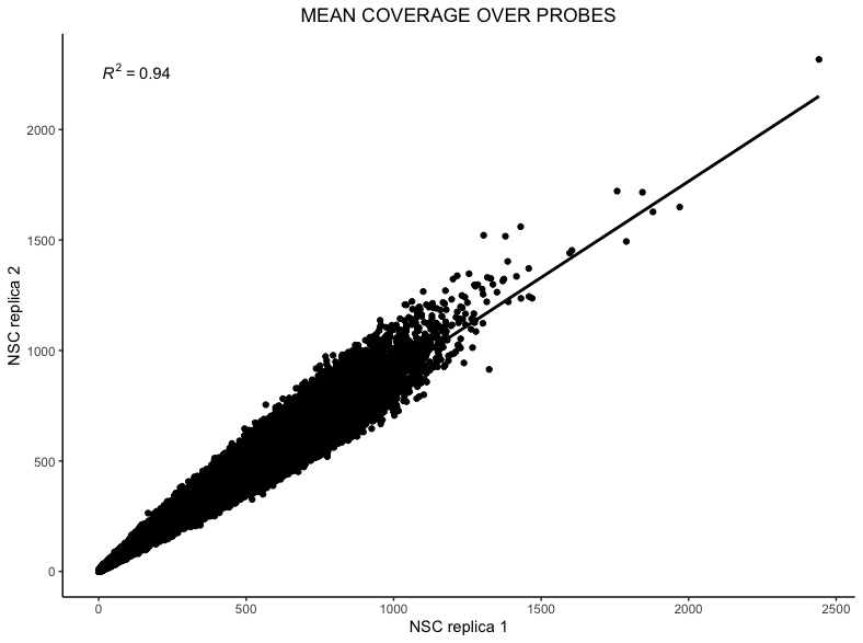
Typically \(R^2\) values for mean probe coverage are around 0.9 (ranging from 0.85 - 0.95) and \(R^2\) values for mean bait coverage are around 0.95 (ranging from 0.95 - 0.99).